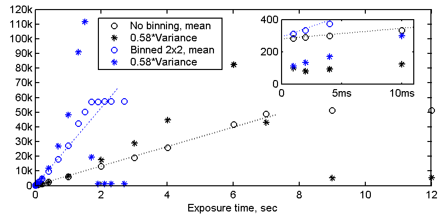
Figure 2. Average readout and variance versus exposure time.
Saturation occurs at 29.7k electrons per pixel in the unbinned mode and 33k electrons per pixel group in the 2x2 binned mode. Again, this is close to the value estimated on the Artemis web page.
The electron gain is defined as the average number of incoming electrons required to increase the readout from the analog to digital converter (ADC) by one count. The gain value is estimated to 0.58 electrons per ADC count.
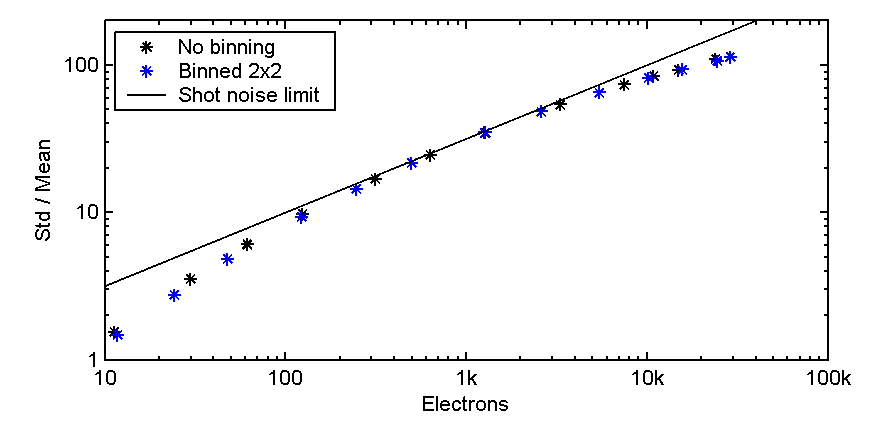
The readout noise is found to be close to the shot noise limit (fundamental noise predicted by quantum theory) for pixel values after dark frame subtraction in the range from 100 to 15k ADC counts (60 to 10k electrons). Below this range the readout noise starts to contribute.
The variance is found to increase faster than expected for shot noise when readout increases above 15k ADC counts. An additional noise seems to be present with a variance that increases with the square of the readout value. This surprises me, and I am curios to find out what the source of this added noise can be. I am also interrested in finding out if this noise is present only in my camera or if it is present in all Artemis (or Art285) cameras.
Close to the full well depth the readout variance is two times higher than the shot noise limit. This implies that two exposures with 40k readout must be stacked to achieve the signal to noise ratio noise level that should in theory be achieved with only one such exposure. This also means that it is not necessarily an advantage in terms of noise to make long exposures with high pixel values at the readout instead of stacking multiple short exposures. For instance, stacking of three 2 minute exposures with 8k readout per pixel should produce about the same signal to noise ratio as one single 10 minute exposures with 40k readout per pixel.
Update
The unexpected incrase in variance at high exposure levels seem to be related to nonlinearity in the camera
responsivity. This may very well mean that the camera noise is dominated only by fundamental and unavoidable
shot noise all the way up to saturation. I will update this page when I have had time to do some more analysis.
The nonlinearity and noise measurements have been discussed in
this thread and
this thread
on the ArtemisCCD group. Note that the earliest posts may contain wrong conclusions.
Results from the linearity test can be found here:
Measured data
Linearity plot
Linearity plot, logaritmic horizontal axis
Linearity was calculated as the ratio between the pixel output values and a linear fit to the
data in the first plot.
All measurements presented below were made in ambient room temperature with the Peltier connected. Firmware version 2.11 and Artemis Capture 2.09 were used with "Amp off" and "In cam precharge subtraction" enabled.
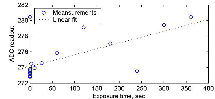
Figure 1 above shows the average readout per pixel versus exposure time with no incoming light. The fitted straight line has a slope of 0.015 ADC counts per second, corresponding to a dark current of 0.009 electrons per second when assuming 0.58 electrons per ADC count.
The mean readout value per pixel is shown as circles in the figure. Saturation occurs at 51.2k ADC counts for unbinned readout, corresponding to a well depth of 29.7k electrons. With 2x2 binned readout saturation occurs at 57k ADC counts, corresponding to a well depth of 33k electrons. Deviation from linearity below saturation is probably mostly due to inaccuracies in the shutter timing, as discussed in this thread on the Yahoo Artemis group. In photometric applications one would measure star intensities relative to one or more reference stars captured in the same frame, to minimize effects of varying atmosphere conditions. This also eliminates errors from exposure timing inaccuracies, and I cannot think of any application where small inaccuracies in exposure timing would cause problems.
The variance of the pixel readout is defined as the average square value of the of the a value from its expectation value or variance when averaged over many exposures. If the variance is the same for all pixels one may alternatively take the difference between two frames and calculate the variance expected from a single readout as 1/2 times the variance of the pixel values within he difference frame. The factor 1/2 must be included because the difference frame contains uncorrelated noise contributions from two different exposures. The use of the difference between two frames instead of a single frame in the calculation suppresses errors related to nonuniformity in the exposure and pixel responsivitity and variations in source intensity from frame to frame. Further improvements can be achieved by scaling the second frame before subtraction so that both frames will have exactly the same mean pixel value. In the figure below I have plotted the calculated variance multiplied by an estimated gain value of 0.58. Te method used for the gain estimation will be explained further down. At this point one may observe that the variance scaled by the gain value has the same slope at low exposures as the mean pixel values.
From the magnified insert plot at the upper right of the figure below the readout offset at zero exposure is estimated to 280 and 292 ADC counts for the unbinned and binned readout, respectively. More interesting, the readout variance at zero exposure is found to be 65/0.58 and 90/0.58 squared ADC units for the two cases, or 65*0.58 and 90*0.58 squared electrons. The readout noise at zero exposure is the square root of these numbers, or 6.1 and 7.2 electrons with unbinned and binned readout, respectively. Again, these measurement was made with ambient room temperature.
Figure 2. Average readout and variance versus exposure time.
This means that if the electron gain (electrons per ADC count) is g and the average number of electrons per pixel is N, then the average ADC readout becomes x = N/g, while the shot noise induced variance of the readout becomes y = N/g2. In addition there will be a bias B in the variance due to readout noise. One should therefore expect the readout variance to vary with the exposure as:
Readout variance y = B + N/g2 = B + x/g.
If shot noise is the only noise component that varies with the exposure, we can estimate the gain parameter g by plotting y versus x and measuring the slope 1/g of this line.
In Figure 3 below the variance from Figure 2 is plotted against the average pixel value. For low exposures (see the insert at upper right in figure) the data follow a linear relation of the form y = b + x/0.58, indicating a gain of g = 0.58 electrons per ADC count. Here, b accounts for both the vertical offset B and for offset in the ADC readout.
The gain parameter has earlier been measured for another Art285 camera with the same method as here to be 0.57, which is very close to my camera. This measurement was done by Tan Thiam Guan (TG) and is discussed here in the ArtemisCCD discussion forum. TG also refers to a report by MiraMetrics , which discusses how errors in measurements of the variance and the gain parameter can be minimized through the use of the scaled frame difference approach described above. The exposure versus variance measured by TG is plotted for exposures up to 6.3k ADC counts in an Excel file ("ART285 Calibration Sheet") stored in the forum's files section, and a nice linear relation is seen.
What surprises me with my own results is that the variance starts to increase faster than the linear curve for pixel values above about 15k ADC counts. The variance fits quite nicely to a quadratic curve which reaches two times the predicted shot noise limit (linear curve) close to the full well capacity. This indicates the presence of a noise mechanism in addition to the shot noise with a standard deviation (not variance) that scales linearly with the ADC readout.
I can only speculate about the origin of this added noise.
The fact that the binned and unbinned measurements show the same trend may
indicate that the added noise does not originate from the ccd array itself.
The noise could be inherent to the ADC, or it could be related to random variations
in the ADC scale factor, which is typically defined by some input reference voltage.
I do not know the shape of the analog ccd signals transferred to the ADC.
However, if the pixel values are transferred as an analog pulse train that returns to
a zero level between each pulse, then clock jitter in the ADC could cause a readout noise
with a standard deviation that increases linearly with the pulse amplitude.
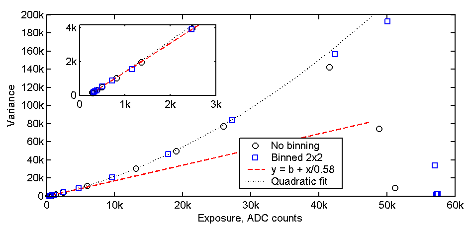
Figure 3. Variance versus average readout.
Figure 4 below summarizes the signal to noise ratio in terms of the standard deviation divided by the average number of recorded electrons.
Erlend Rřnnekleiv, www.eronn.net erlend.web&eronn.net [replace & with @]